The KISS principle in machine learning
Tags: projects, research
Software developers are already familiar with the KISS principle. Roughly speaking, it refers to the old wisdom that simple solutions are to be preferred, while unnecessary complexity should be avoided. In machine learning, this means that one should increase the complexity iteratively, starting from simple models and—if necessary—working upwards to more complicated ones. I was recently reminded and humbled by the wisdom of KISS while working on a novel topology-based kernel for machine learning.
Prelude: A Paper on Deep Graph Kernels
A recent paper by Yanardag and Vishwanathan introduced a way of combining graph kernels with deep learning techniques. The new framework basically yields a way of using graph kernels, such as graphlet kernels in a regular deep learning setting.
The two researchers used some interesting data sets for their publication. Most notably, they extracted a set of co-occurrence networks (more about that in a minute) from Reddit, a content aggregation and discussion site. Reddit consists of different communities, the subreddits. Each subreddit deals with a different topic, ranging from archaeology to zoology. The posting style of these subreddits varies a lot. There are several subreddits that are based on a question–answer format, while others are more centred around individual discussions.
Yanardag and Vishwanathan hence crawled the top submissions from the subreddits IamA, AskReddit, both of which are based on questions and answers, as well as from TrollXChromosomes, and atheism, which are discussion-based subreddits. From every submission, a graph was created by taking all the commenters of a thread as nodes and connecting two nodes by an edge if one user responds to the comment of another user. We can see that this is an extremely simple model—it represents only a fraction of the information available in every discussion. Nonetheless, there is some hope that qualitatively different behaviours will emerge. More precisely, the assumption of Yanardag and Vishwanathan is that there is some quantifiable difference between question–answer subreddits and discussion-based subreddits. Their paper aims to learn the correct classification for each thread. Hence, given a graph, we want to teach the computer to tell us whether the graph is more likely to arise from a question–answer subreddit or from a discussion-based one.
The two researchers refer to this data set as REDDIT-BINARY. It is now available in a repository of benchmark data sets for graph kernels, gracefully provided and lovingly curated by the CS department of Dortmund University.
Interlude: Looking at the Data
Prior to actually working with the data, let us first take a look at it in order to get a feel for its inherent patterns. To this end, I used Aleph, my library for topological data analysis read and convert the individual graphs of every discussion to the simpler GML format. See below if you are also interested in the data. Next, I used Gephi to obtain a force-directed visualization of some of the networks.
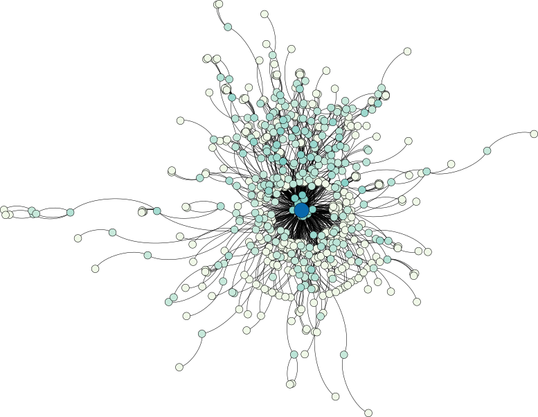
A look at a question–answer subreddit shows a central core structure of the data set, from which numerous strands—each corresponding most probably to smaller discussions—emerge:
The discussion-based subreddit graph, on the other hand, exhibits a larger depth, manifesting themselves in a few long strands. Nonetheless, a similar central core structure is observable as well.
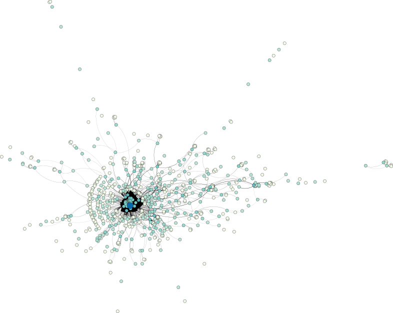
Keep in mind that the selected examples are not necessarily representative—I merely picked two of the large graphs in the data set to obtain an idea of how the data looks.
A Complex Classification
A straightforward way to classify those networks would be to use graph kernels, such as the graphlet kernels. The basic idea behind these kernels is to measure a dissimilarity between two graphs by means of, for example, the presence or absence of certain subgraphs. At least this is the strategy pursued by the graphlet kernel. Other kernels may instead opt for comparing “random walks” on both graphs. A common theme of these kernels is that they are rather expensive to compute. In many applications, they are the only hope of obtaining suitable dissimilarity information without having to solve the graph isomorphism problem, which is even more computationally expensive. Hence, graph kernels are often the only suitable way of assessing the dissimilarity between graphs. They are quite flexible and, as the authors show, can even be integrated into a deep learning framework.
As for their performance, Yanardag and Vishwanathan report an accuracy of 77.34% (standard deviation 0.18) for graphlet kernels and 78.04% (standard deviation 0.39) for deep graphlet kernels, which is very good considering the baseline for random guessing is 50%.
A Simple Classification
In line with the KISS principle, I wanted to figure out alternative ways of achieving similar accuracy values with a better performance, if possible. This suggests a feature-based approach with features that can be calculated easily. There are numerous potential options for choosing these features. I figured that good choices include the “average clustering coefficient” of the graph, the “average degree”, the average shortest path length, the “density”, and the “diameter” of the graph. Among these, the average shortest path length and the diameter take longest to compute because they essentially have to enumerate all shortest paths in the graph. So I only used the remaining three features, all of which are computable in polynomial time.
I used the excellent NetworkX package for Python to do most of the heavy lifting. Reading a graph and calculating its features is as easy as it gets:
import networkx as nx

G = nx.read_gml(filename, label='id')

average_clustering_coefficient = nx.average_clustering(G)
average_degree                 = np.mean( [degree for _,degree in nx.degree(G) ] )
density                        = nx.density(G)
I collect these values in a pandas.DataFrame to simplify their handling. Now
we have to choose some classifiers. I selected decision trees, support vector machines, and logistic regression. Next, let us train and test each of these classifiers by means of 10-fold “cross-validation”.
X = df.values
y = labels

classifiers = [ DecisionTreeClassifier(), LinearSVC(), LogisticRegression() ]
for clf in classifiers:
  scores = cross_val_score(clf, X, y, cv=10)
  print("Accuracy: %0.4f (+/- %0.2f)" % (scores.mean(), scores.std() * 2))
As you can see, I am using the default values for every classifier—no grid search or other technique for finding better hyperparameters for now. Instead, I want to see how these classifiers perform out of the box.
Astonishing Results
The initial test resulted in the following accuracy values: 77.84% (standard deviation 0.16) for decision trees, 64.14% (standard deviation 0.45) for support vector machines, and 55.54% (standard deviation 0.49) for logistic regression. At least the first result is highly astonishing—without any adjustments to the classifier whatsoever, we obtain a performance that is en par with more complex learning strategies! Recall that Yanardag and Vishwanathan adjusted the hyperparameters during training, while this approach merely used the default values.
Let us thus focus on the decision tree classifier first and figure out why it performs the way it did. To this end, let us take a look at what the selected features look like and how important they are. To do this, I just added a single training instance, based on standard test–train split of the decision tree classifier:
X_train, X_test, y_train, y_test = train_test_split(X,y, test_size=0.20)

clf = DecisionTreeClassifier()
clf.fit(X_train, y_train)

print(clf.feature_importances_)
This results in [ 0.18874114 0.34113588 0.47012298 ], meaning that
all three features are somewhat important, with density accounting for
almost 50% of the purity of a node—if you are unfamiliar with
decision trees, the idea is to obtain nodes that are as
“pure” as possible, meaning that there should be as few
differences in class labels as possible. The density attribute appears
to be important for splitting up impure nodes correctly.
To get a better feeling of the feature space, let us briefly visualize it using “principal component analysis”:
clf = PCA(n_components=2)
X_  = clf.fit_transform(X)

for label in set(labels):
  idx = y[0:,] == label
  plt.scatter(X_[idx, 0], X_[idx, 1], label=label, alpha=0.25)

plt.legend()
plt.show()
This results in the following image:

Every dot in the image represents an individual graph, whereas distances in the plot roughly correspond to distances between features. The large amount of overlaps between graphs with different labels thus seems to suggest that the features are insufficient to separate the individual graphs. How does the decision tree manage to separate them, nonetheless? As it turns out, by creating a very deep and wide tree. To see this, let us export the decision tree classifier:
with open("/tmp/clf.txt", "w") as f:
  export_graphviz(clf, f)
Here is a small depiction of the resulting tree:
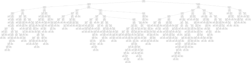
There is also a larger variant of this tree for you to play around with. As you can see, the tree looks relatively complicated, so it is very much tailored to the given problem. That is not to say that the tree is necessarily suffering from overfitting—we explicitly used cross-validation to prevent this. What it does show is that the simple feature space with three features, while yielding very good classification results, is not detecting the true underlying structure of the problem. The rules generated by the decision tree are artificial in the sense that they do not help us understand what makes the two groups of graphs different from each other.
Coda
So, where does this leave us? We saw that we were able to perform as well as state-of-the-art methods by merely picking a simple feature space, consisting of three features, and a simple decision tree classifier. I would say that any classifier with a higher complexity should yield significant improvements over this simple baseline, both in terms of average accuracy and in terms of standard deviation. Hence, the KISS principle in machine learning: start simple and only add more complex building blocks, i.e. models, if you have established a useful baseline.
You can find both the code and the data in my repository on topological machine learning. To run the analysis described in this blog post, just execute
$ ./simple_network_analysis.py GML/????.gml Labels.txt
in the REDDIT-BINARY subfolder of the repository.
That is all for now, until next time!