Towards Shakespearean Social Network Analysis
Tags: projects, research
gdb »
I recently had the pleasure to see a talk about the style of Shakespeare, given by Prof. Dr. Beatrix Busse and her inspired staff. One of the talks, given by Ingo Kleiber, struck a nerve in me. He talked about creating social networks from Shakespeare’s plays and analyse them in the way we analyse, well, “real” social networks.
Naturally, I needed to see for myself how fun this would be. In the subsequent sections, I am going to describe some initial considerations. I plan on neglecting my dissertation for a little bit to present a more concise write-up later on.
Where to get some data?
Luckily for us, many people have already invested large chunks of their time to make Shakespeare’s plays accessible and readable for computers. There is a whole corpus of 37 plays, in a computer-readable format, available for download. Hence, no need to do any “natural language processing” for now.
What do with it?
Some gentle prodding with Python makes it possible to extract a “co-occurrence network” from the play. How this extraction is done is somewhat subjective. In my initial attempt, following the analysis made by Ingo, I broke down the plays in individual scenes. After identifying the characters in every scene, I opted for adding an edge between two characters if they appear in the same scene. Of course, this is somewhat rough—we may never know whether they actually talk to each other. Also, I did not yet take stage directions into account. It is thus well possible that I add an edge between two characters that are never actually on the stage at the same time. This obviously needs to be improved for any “serious” analysis—from which I am very far removed anyway, by virtue of being a barbarian in the ways of linguistics!
So, having extracted all those edges, I decided on building a “adjacency matrix” where edge weights indicate how often characters are part of the same scene. This permits me to draw really nice network diagrams, such as this one here (which comes from Macbeth, one of my most favourite plays):

Nodes have been scaled and coloured according to their degree, just like the edges. The darker the colour, the more important the character. Not too surprisingly, Macbeth itself appears to be important to this play. Who could have anticipated this? The graph layout algorithm—a simple force-directed scheme—also serves to separate the play quite well. The parts with the “Weird Sisters” are clearly shown to be somewhat different from the rest of the action.
Density
While this looks nice and all, it is not exactly informative. We need to compare more plays with and among each other! To do just that, I calculated the graph density—the ratio between the actual amount of edges and the total number of possible edges—for every play. The graph density measures how, well, dense the graph is in terms of edges. In other words, the more the graph resembles a complete graph, the higher its density will be. In theatrical terms, I imagine that a dense co-occurrence network indicates many plot lines that are interwoven and converge later on, prompting literally every character to be connected to the other characters.
To perform some exploratory data analysis on Shakespeare’s plays, let us take all plays, tag them according to three types (comedy, tragedy, and history), which the corpus fortunately provides on its own, and plot graph density against the number of characters. This is how it looks like:
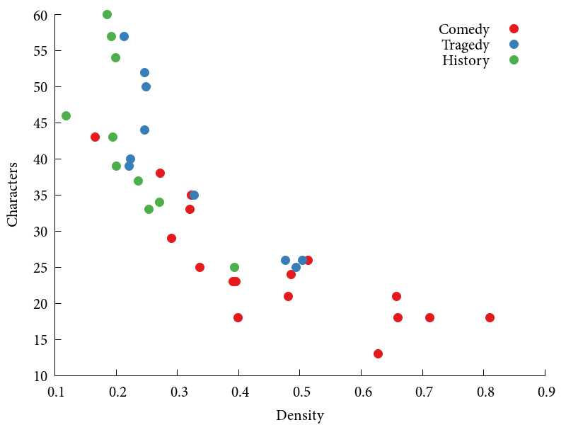
Finally, some nice patterns! Notice that all the historical plays—such as Henry V—are characterized by having a rather low density (less than 0.4) but, for the most part, a large amount of characters. The comedies, by contrast, have a lower amount of characters and a substantially higher density. The most dense play, in this representation, is Love’s Labour’s Lost, one of Shakespeare’s early comedies. The most sparse one is Pericles, Prince of Tyre, where the authorship of Shakespeare is somewhat unclear.
What to make of this?
It is certainly interesting to see that some patterns start to emerge when one uses statistical or data analysis techniques to analyse a whole corpus of works. There are lots of interesting applications here. I did not include any dates, for example. How do the works change over time? Are plays of later Shakespearean periods less dense or more dense?
I am very much looking forward to doing more with these data.
Since I did not release any code so far, please take a look at Ingo’s repository, where he thankfully provides his sample code to create social networks from the plays.
Let the age of Bard Data begin!