Volume rendering for DICOM images
Tags: programming, software, projects, visualization
I always wanted to look inside my own head. During the last few years, I was given the opportunity to do so. On several occasions, doctors took some “MRI” images of my head (there is nothing wrong with my head—this was the standard operating procedure in some situations). Some time later, they also took “MRA” images, meaning that I got to see my grey matter and my blood vessels. Even better, the doctors were only happy to provide me with the raw data from their examinations. A true treasure for a visualization scientists, as both MRI and MRA result in “Voxel data” that may be visualized by “volume rendering techniques”. In mathematical terms, I wanted to visualize a 3-dimensional scalar field in a cubical volume. In Hollywood terms, I wanted a program to zoom into my brain and take a look at my blood vessels.
This post describes how I went from a stack of DICOM images to a set of raw volume data sets that can be visualized with ParaView, for example.
The setup
The German healthcare system being what it is, I quickly received a bunch of DVDs with my
images. The DVDs contained some sort of Java-based viewer application, developed by CHILI
GmbH. Unfortunately, medical laypersons such as myself
are probably not the targeted user group for this software—I thus decided that it
would be easier to rely on other tools for visualizing my head. A quick investigation
showed that the data are ordered in a hiearchy such as DATA/PAT/STUD??/SER??/IMG???. The
STUD part refers to the examination that was performed, e.g. an MRI of a certain part of
the head. Each SER part contains up to (in my case) 33 different directories with the
results of a single series of the MRI/MRA. Each subdirectory consists of lots of single
images in “DICOM format”.
DICOM describes a standard for exchanging information in medical imaging. It is rather complicated, though, so I used the ImageJ image processing program, to verify that each of the images describes a slice of the MRI/MRA data. To obtain a complete volume from these image, I had to convert them into a single file. Luckily, some brave souls have spent a considerable amount of time (and, I would expect, a sizeable amount of their sanity, as well) to write libraries for parsing DICOM. One such library is pydicom, which permits reading and (to a limited extent) writing DICOM files using Python. It is currently maintained by Darcy Mason. Since pydicom’s documentation is rather raw at some places, I also perused Roni’s blog “DICOM is easy” to grasp the basics of DICOM. It turned out that each of the DICOM files contains a single entry with raw pixel data. Since all images of a given series should have the same dimensions, I figured that it would be possible to obtain a complete volume by extracting the raw data of each image and concatenating them. I wrote multiple Python scripts for doing these jobs.
Sample data
If you do not have any DICOM images at your disposal, I would recommend visiting the
homepage of Sébastien Barré and download the
CT-MON2-16-brain file, for example. I would very much like to include some sample files
in the repository of the scripts, but I am not sure how these samples are licenced, so I
prefer linking to them.
dicomdump.py
This script extracts the “pixel data” segment of a DICOM file while writing some
information to STDERR:
$ ./dicomdump.py CT-MONO2-16-brain > CT-MONO2-16-brain.raw
##############
# Pixel data #
##############

Width:                      512
Height:                     512
Samples:                    1
Bits:                       16
Photometric interpretation: MONOCHROME2
Unsigned:                   0
You should now be able to read CT-MONO2-16-brain.raw using ImageJ, for example.
dicomcat.py
This script concatenates multiple images from a series of DICOM files to form a volume.
Assuming you have files with a prefix of IMG in the current directory, you could do the
following:
$ ./dicomcat.py IMG* > IMG.raw
[ 20.00%] Processing 'IMG001'...
[ 40.00%] Processing 'IMG002'...
[ 60.00%] Processing 'IMG003'...
[ 80.00%] Processing 'IMG004'...
[100.00%] Processing 'IMG005'...
Finished writing data to '<stdout>'
Using the optional --prefix parameter, you can also create an output file automatically:
$ ./dicomcat.py --prefix IMG Data/2011/STUD02/SER01/IMG00*
[ 20.00%] Processing 'IMG001'...
[ 40.00%] Processing 'IMG002'...
[ 60.00%] Processing 'IMG003'...
[ 80.00%] Processing 'IMG004'...
[100.00%] Processing 'IMG005'...
Finished writing data to 'IMG_320x320x5_16u'
The file names generated by the script follow the same pattern. The first three numbers indicate the dimensions of the volume, i.e. width, height, and depth. The last digits indicate the number of bits required to read the image and whether the data are signed (indicated by s) or unsigned (indicated by u). The example file is thus a volume of width 320, height 320, and depth 5, requiring 16 bit unsigned integers for further processing.
recursive_conversion.py
This script converts the aforementioned directory hierarchy. Just point it towards a root
directory that contains subdirectories with series of images and it will automatically
create raw images. For example, assuming that you have folders SER1, SER2, and SER3
in the folder STUD. To concatenate all images in all of these folders automatically,
call the script as follows:
$ ./recursive_conversion.py STUD
[ 20.00%] Processing 'IMG001'...
[ 40.00%] Processing 'IMG002'...
[ 60.00%] Processing 'IMG003'...
[ 80.00%] Processing 'IMG004'...
[100.00%] Processing 'IMG005'...
Finished writing data to 'SER1_320x320x20_16u'
[...]
Finished writing data to 'SER2_320x320x15_16u'
[...]
Finished writing data to 'SER3_512x512x10_16u'
Viewing the volume
The easiest option for viewing the volume is ParaView. Open the file
using the “Raw (binary)” file type. In the “Properties” section of the data set, enter the correct
extents. A 352x512x88 file, for example, has extents of 351x511x87, respectively. Choose
“Volume” in the “Representation” section and play with colour map until you see the structures you
want to see.
This is what it looks like:
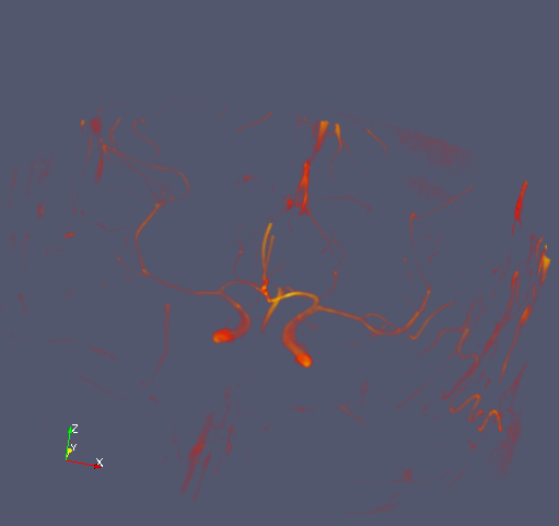
Blood vessels in my brain. If I were a neurologist, I could probably name them as well. Hazarding a guess, I would say that the prominent structure is probably the carotid artery.
Code
The code is released under the “MIT Licence”. You may download the scripts from their git repository.