Eigenfaces reconstructions
Tags: programming
While learning about “principal component analysis” for the first time, I also encountered the intriguing world of eigenfaces. Briefly put, back in the mists of time—at least in computer science terms—Matthew Turk and Alex Pentland came up with an ingenious approach towards face recognition and classification. At it’s core, the method consists of nothing but an eigenvalue decomposition. Let me briefly outline the steps:
- Acquire a set of images showing faces. I am assuming that the images are grey-scale because this means that we do not have to think about different colour channels.
- Treat each digital image as a vector in a high-dimensional space by “flattening” the image vector. An image of dimensions 192 ×64 pixels becomes a 12288-dimensional vector, for example.
- Calculate the mean face of the data set and subtract it from all images. This corresponds to centring the distribution of faces.
- Put all vectors into a matrix. The result is a matrix with as many rows as the dimensions of the faces, and as many columns as there are faces.
- Calculate the eigenvalue decomposition of the sample covariance matrix. This step hides a clever trick: We do not calculate the sample covariance matrix of the original matrix, which would be a square matrix with the row dimension of the original data, for example 12288 ×12288. Instead, we calculate the transpose of this matrix, which uses the column dimension of the original data. This matrix will hence only have as many rows and columns as there are faces in the data. It can be shown that an any eigenvector of this matrix multiplied with the original matrix yields an eigenvector of the large covariance matrix.
- Of course, we do not use all eigenvalues and eigenvectors but rather only as many until we have reached, say, 95% of explained variance. This removes a surprisingly large amount of data.
- If we have the reduced eigensystem, we can project any new face to the (reduced) basis of eigenvectors. This allows us to embed them in what Turk and Pentland call the “face space”.
- The projection permits us to decide whether something is a face at all by checking whether it is sufficiently close to the other vectors in “face space”. Furthermore, it permits face classification by assigning a known face to its nearest neighbour (or to its nearest class of faces). These operations only require basic vector multiplication operations, so they are very cheap.
Such a pretty neat algorithm deserves a neat implementation. I tried to write one myself in Python. You can find the code in the Eigenfaces repository on my GitHub profile. As always, it is licensed under an MIT license. Note that the script currently only supports the reconstruction aspect of faces. It will randomly partition input data into training and test data, perform the eigensystem calculations on the training data, and attempt the reconstruction on the test data.
I used a classical database of faces, the Yale faces data, which has been preprocessed by some nice folks at MIT. In the repository, I only included the original and cropped variants of the faces—the preprocessed data set contains much more.
The results are interesting and highlight some of problems with the approach. Since the eigendecomposition is completely agnostic concerning any sorts of facial features, it may “learn” the wrong thing. Input data needs to be chosen carefully and should ideally be already cropped. Otherwise, the reconstruction quality is not very great. For example, this happens when I train on 100 out of 165 images with 95% explained variance:
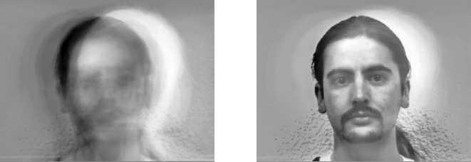
We can see that our reconstruction (left) captures mostly the uninteresting stuff, namely the position of the head, as well as some lighting details, in comparison to the original (right). Here”s a similar example with the cropped faces:
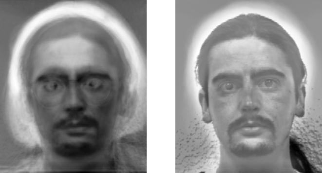
This version is much better. Of course, it also contains the ghostly remains of the glasses, but all in all, the reconstruction is more true to the original.
For such a conceptually simple algorithm, these are rather nice results. It is very intriguing to see how well even simple classifiers can perform. If you want to play with the algorithm yourself, please grab a copy of the repository.